Electromechanical System, Electric Machines, and Applied Mechatronics

Presentation on theme: "Electromechanical System, Electric Machines, and Applied Mechatronics"— Presentation transcript:

1 Electromechanical System, Electric Machines, and Applied Mechatronics
CONTENTS 7.4 Conventional three-phase syncronous machines; Dynamics in the machine variables,and in the rotor And syncronous reference frames 7.4.1 Dynamics of synchronous machines in the machine variables 7.4.2 Mathematical models of synchronous macines in the rotor and synchronous reference frames

2 7.4.1 Dynamics of snchronous machines in the machine variavles,
and in the rotor and synchronous reference frame

3 Voltage equation for stator windings and rotor windings
Uas, ubs,and ucs, are the phase voltages in the stator windings as,bs,and cs, respectively Ias,ibs,and ics,are the phase currents in the stator windings as,bs,and cs, respectively are the stator flux linkages Ufr is the exitation voltage applide to the rotor winding fr is the rotor flux linkage rs and rr are the resistances of the stator and rotor windings, respectively

4 Stator and Rotor flux linkages
Self component

5 Define , 1. Salient type 2. Round-rotor type
 The magnetic paths in the quadrature and direct magnetic axes are idntical

6 Matrix of self-and mutual Inductances
Self inductance

7 Vector Matrix of flux linkage

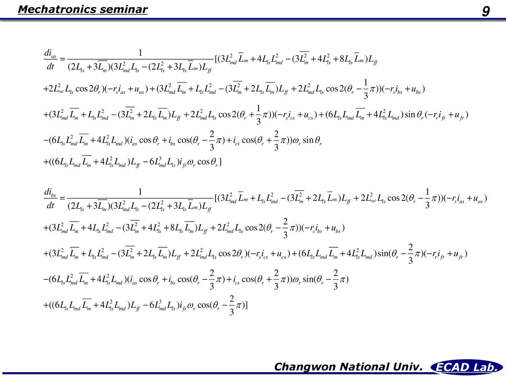
8 Voltage equation for stator windings and rotor windings

9

10

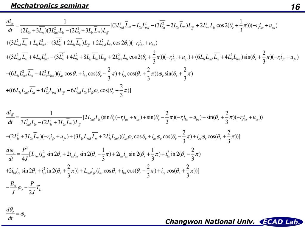
11 The torsional-mechanical equation

12 Relation of mechanical(wrm) and electrical velocity (wrm)
according to Pole number

13 The electromagnetic Torque

14 The torsional-mechanical equation

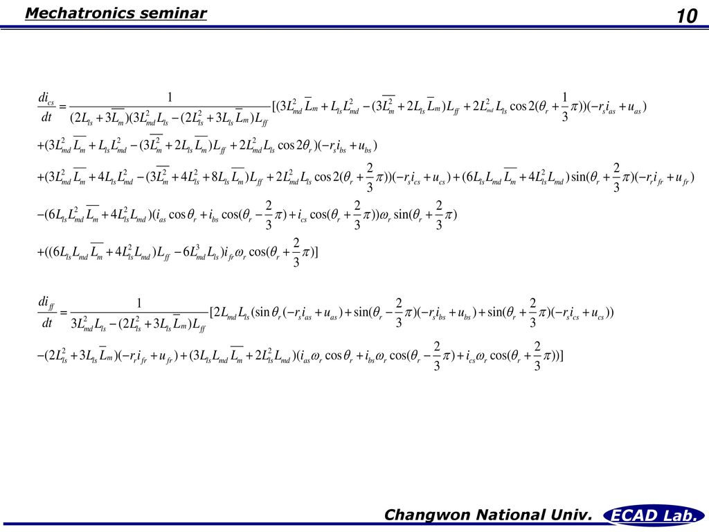
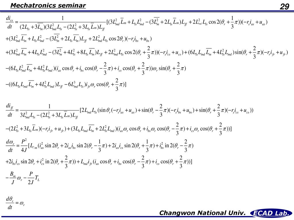
15 The nonlinear differential equations to map the transient dynamics of three-phase synchronous motors

16

17 Torque equation except viscous friction coefficient (Bm)

18 Typical torque-speed characteristic curves of synchronous motors

19 Example 7.6 Model a three-phase, two-pole synchronous motor with following parameters parameters 값 단위 Rs 0.25 [ohm] Rr 0.47 [H] Lls 0.0001 Lmq Lmd Llf Lmf J 0.003 [Kg-m2] Bm [N-m-s-rad-1]

20 The field voltage is ufr=5V
The load conditions are specified as

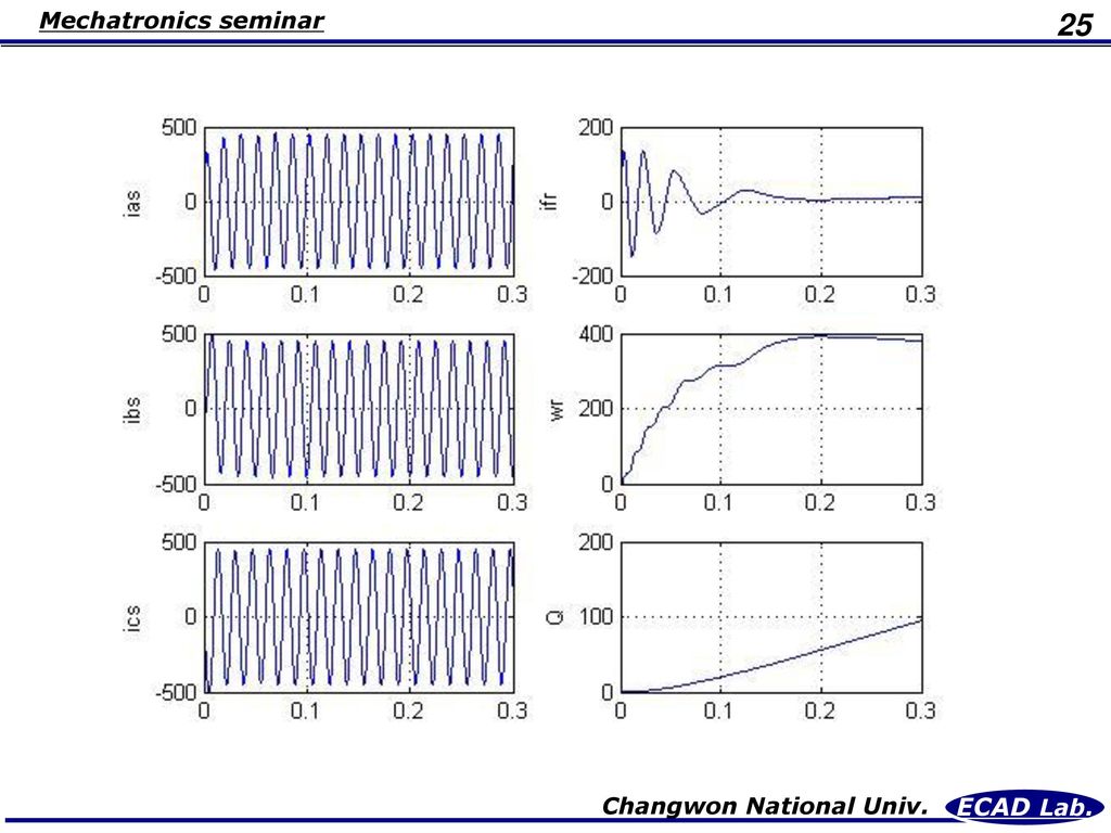
21 MATLAB script crm_01.m tspan=[0 0.5];y0=[0 0 0 0 0 0]';
options=odeset('RelTol',5e-3,'AbsTol',[1e-4 1e-4 1e-4 1e-4 1e-4 1e-4]); [t,y] = ODE45('crm_02',tspan,y0,options); subplot(3,2,1); plot(t,y(:,1)); ylabel('ias'); axis([0,0.3,-500,500]); grid; subplot(3,2,3); plot(t,y(:,2)); ylabel('ibs'); axis([0,0.3,-500,500]); grid; subplot(3,2,5); plot(t,y(:,3)); ylabel('ics'); axis([0,0.3,-500,500]); grid; subplot(3,2,2); plot(t,y(:,4)); ylabel('ifr'); axis([0,0.3,-200,200]); grid; subplot(3,2,4); plot(t,y(:,5)); ylabel('wr'); axis([0,0.3,0,400]); grid; subplot(3,2,6); plot(t,y(:,6)); ylabel('Q'); axis([0,0.3,0,200]); grid;

22 MATLAB script crm_02.m function yprime=difer(t,y);
Lls=0.0001;Lmqs= ;Lmds= ; Llf= ;Lmf=0.0001; Lmd= ; Lmb=(Lmqs+Lmds)/3; rs=0.25;rr=0.47; J=0.003;Bm= ; P=2; um=sqrt(2)*150;w=377; ufr=5; if t<=0.2; T1=0; else T1=1; end

23 uas=um*cos(w*t); ubs=um*cos(w*t-2*pi/3); ucs=um*cos(w*t+2*pi/3); Ld=2*Lls*Lmd^2;Ldr=2*Lls*Lmd; Lss=(-3*Lmb^2-4*Lls^2-8*Lls*Lmb)*(Lmf+Llf)+3*Lmd^2*Lmb+4*Lls*Lmd^2; Ldens=(2*Lls+3*Lmb)*((-2*Lls^2-3*Lmb*Lls)*(Llf+Lmf)+3*Lmd^2*Lls); Ldenr=(-2*Lls^2-3*Lmb*Lls)*(Llf+Lmf)+3*Lmd^2*Lls; Lms=(-3*Lmb^2-2*Lls*Lmb)*(Lmf+Llf)+3*Lmd^2*Lmb+Lls*Lmd^2; Lrr=6*Lls*Lmd*Lmb+4*Lls^2*Lmd; Llr=-(2*Lls^2+3*Lmb*Lls); S1=sin(y(6,:)); S2=sin(y(6,:)-2*pi/3);S3=sin(y(6,:)+2*pi/3); IUas=-rs*y(1,:)+uas;IUbs=-rs*y(2,:)+ubs;IUcs=-rs*y(3,:)+ucs; IUfr=-rr*y(4,:)+ufr; C1=cos(y(6,:));C2=cos(y(6,:)-2*pi/3);C3=cos(y(6,:)+2*pi/3); C12=cos(2*y(6,:));C22=cos(2*y(6,:)-2*pi/3);C32=cos(2*y(6,:)+2*pi/3); Nsts=(-6*Lmd^2*Lls*Lmb-4*Lmd^2*Lls^2)*y(5,:).*(C1.*y(1,:)+C2.*y(2,:)+ C3.*y(3,:)); Nstr=(3*Lmd*Lmb*Lls+2*Lmd*Lls^2)*y(5,:).*(C1.*y(1,:)+C2.*y(2,:)+C3.*y(3,:)); Nct=((6*Lmd*Lls*Lmb+4*Lmd*Lls^2)*(Llf+Lmf)-6*Lmd^3*Lls)*y(5,:).*y(4,:); Te=P*(Lmd*y(4,:).*(y(1,:).*C1+y(2,:).*C2+y(3,:).*C3))/2;

24 yprime=[((Lss+Ld. C12). IUas+(Lms+Ld. C22). IUbs+(Lms+Ld. C32)
yprime=[((Lss+Ld*C12).*IUas+(Lms+Ld*C22).*IUbs+(Lms+Ld*C32).*IUcs+Lrr*S1.*IUfr+Nsts.*S1+Nct.*C1)/Ldens;... ((Lms+Ld*C22).*IUas+(Lss+Ld*C32).*IUbs+(Lms+Ld*C12).*IUcs+Lrr*S2.*IUfr+Nsts.*S2+Nct.*C2)/Ldens;... ((Lms+Ld*C32).*IUas+(Lms+Ld*C12).*IUbs+(Lss+Ld*C22).*IUcs+Lrr*S3.*IUfr+Nsts.*S3+Nct.*C3)/Ldens;... (Ldr*S1.*IUas+Ldr*S2.*IUbs+Ldr*S3.*IUcs+Llr*IUfr+Nstr)/Ldenr;... (P*Te-2*Bm*y(5,:)-P*T1)/(2*J);... y(5,:)];

25

26 Dynamics of three-phase synchronous generators

27 Voltage equation for stator windings and rotor windings

28 The nonlinear differential equations to map the transient dynamics of three-phase synchronous generators

29

30 7.4.2 Mathematical models of synchronous machines in the rotor
and synchronous referencd frames -교류 전동기는 전동기의 인덕턴스가 전동기 속도에 관한 함수로 나타난다 -교류 전동기의 전압 방정식은 전동기가 정지하고 있는 경우를 제외하면, 시변 미분 방정식으로 나타나게 된다 변수의 변환은 이러한 복잡한 시변 미분 방정식을 보다 쉽게 해석하기 위함 3상 교류 전동기의 a,b,c상의 변수들을 d,q,n의 직교 좌표계상의 변수로 변환 D축:여자자속이 존재하는축 , q축:d축과 직각을 이루는 축 N축:d-q축과 3차원 공간 상에서 서로 직교하는 축(회전자계의 형성에는 기여하지 않는다)

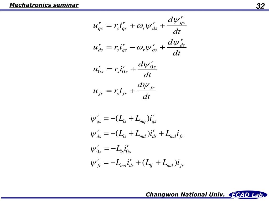
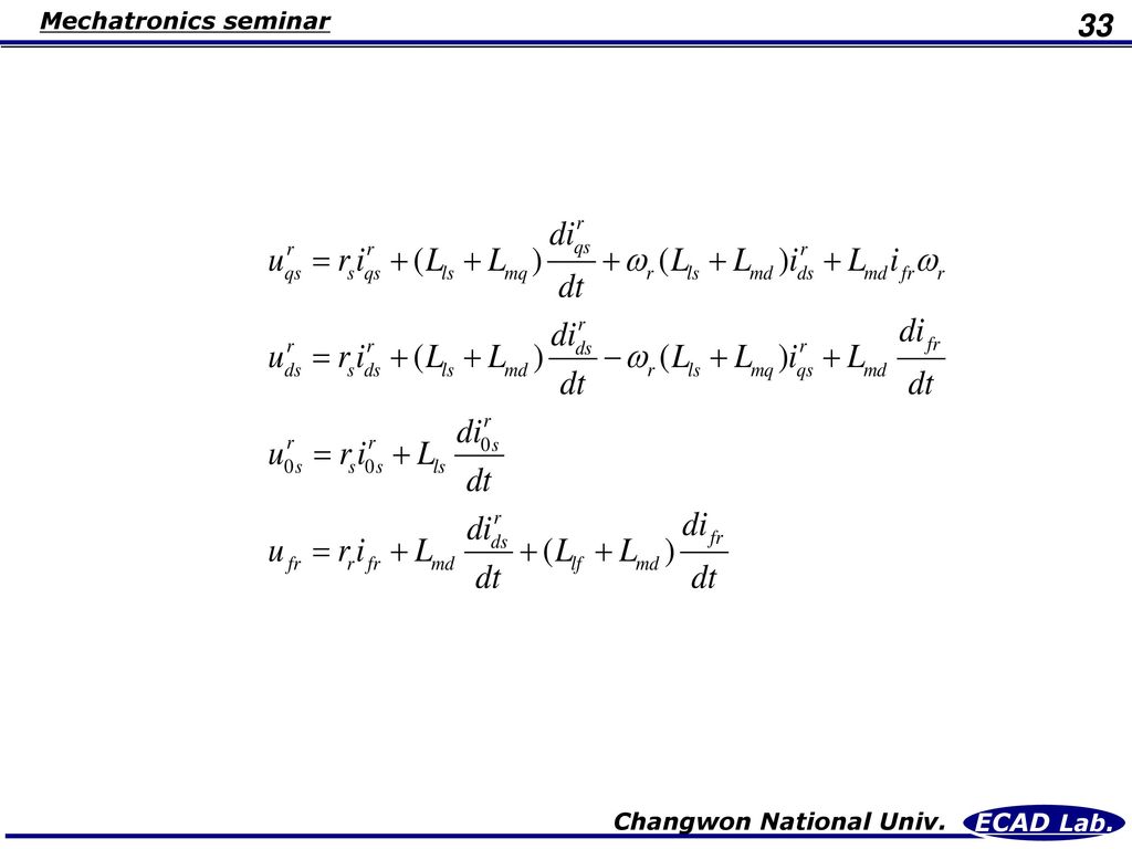
31 The Park transformation
Making use of the Park transformation The rotor reference frame

32

33

34 The electromagnetic torque by using the Park transformation
The torsional-mechanical dynamics for conventional synchronous motors