Principal Component Analysis

Principal Component Analysis
Lecture Notes By Gun Ho Lee Intelligent Information Systems Lab Soongsil University, Korea 1 1

Outline of lecture What is feature reduction ? Why feature reduction?
Basic Idea of Feature Reduction Feature reduction algorithms Principal Component Analysis Nonlinear PCA using Kernels

X A Feature Reduction ? P variables K variables n n data data
학습 데이터를 이용하여 매개 변수를 추정하고 그것을 이용하여 특징 추출함 정보 손실을 최소화하는 조건에서 차원 축소 Karhunen-Loeve (KL) 변환 또는 Hotelling 변환이라고도 부름 혹은 data reduction, dimension reduction n data P variables A n data K variables X

High-dimensional data
Gene expression Face images Handwritten digits

Feature Reduction balancing act between
clarity of representation, ease of understanding oversimplification: loss of important or relevant information.

Why feature reduction? Most machine learning and data mining techniques may not be effective for high-dimensional data Curse of Dimensionality Query accuracy and efficiency degrade rapidly as the dimension increases. The intrinsic dimension may be small. For example, the number of genes responsible for a certain type of disease may be small.

Why feature reduction? 벡터의 차원이 높아짐에 따라 생길 수 있는 문제점
Feature수가 많으면 noise feature가 포함되므로 오히려 분류에 정확성을 저해. Feature수가 많으면 패턴 분류기에 의한 학습과 인식 속도가 느려진다. Feature수가 많으면 모델링에 필요한 학습 집합의 크기가 커진다. PCA는 고차원 특징 벡터를 저차원 특징 벡터로 축소하는 특징 벡터의 차원 축소(dimension reduction) 뿐만 아니라 데이터 시각화 그리고 특징 추출에도 유용하게 사용되는 데이터 처리 기법 중의 하나임.

Why feature reduction? Visualization: projection of high-dimensional data onto 2D or 3D. Data compression: efficient storage and retrieval. Noise removal: positive effect on query accuracy.

Application of feature reduction
Face recognition Handwritten digit recognition Text mining Image retrieval Microarray data analysis Protein classification Interpretation Pre-processing for regression Classification Noise reduction Pre-processing for other statistical analyses

Application of feature reduction
Process monitoring Sensory analysis (tasting etc.) Product development and quality control Rheological measurements Process prediction Spectroscopy (NIR and other) Psychology Food science Information retrieval systems Consumer studies, marketing

Basic Idea of Feature Reduction
정보 손실의 공식화 원래 훈련 집합이 가진 정보란 무엇일까? 샘플들 간의 거리, 그들 간의 상대적인 위치 등 그림의 세 가지 축 중에 어느 것이 정보 손실이 가장 적은가? PCA는 샘플들이 원래 공간에 ‘퍼져있는 정도를’ 변환된 공간에서 얼마나 잘 유지하느냐를 척도로 삼음 이 척도는 변환된 공간에서 샘플들의 분산으로 측정함 이러한 아이디어에 따라 문제를 공식화 하면, 변환된 샘플들의 분산을 최대화 하는 축 (즉 단위벡터 a)을 찾아라.

Basic Idea of Feature Reduction
Representation of feature reduction 차원 축소의 표현 D 차원 단위벡터 a 축으로의 투영

Basic Idea of Feature Reduction Principal Component Analysis Geometric Rationale of PCA Nonlinear PCA using Kernels

Geometric Rationale of PCA
objects are represented as a cloud of n points in a multidimensional space with an axis for each of the p variables the centroid of the points is defined by the mean of each variable the variance of each variable is the average squared deviation of its n values around the mean of that variable. Variance: 16 16

degree to which the variables are linearly correlated is represented by their covariances. Mean of variable i Value of variable j in object m Covariance:

Algebraic definition of PCA
Given a sample of n observations on a vector of p variables define the first principal component of the sample by the linear transformation where the vector is chosen such that is maximum.

Example) Variance 1.0 variance 1.0938 더 좋은 축이 있나? 예제) 변환 공간에서의 분산
Sample data Variance 1.0 variance 더 좋은 축이 있나?

Objective of PCA is to rigidly rotate the axes of this p-dimensional space to new positions (principal axes) that have the following properties: ordered such that principal axis 1 has the highest variance, axis 2 has the next highest variance, .... , and axis p has the lowest variance covariance among each pair of the principal axes is zero (the principal axes are uncorrelated).

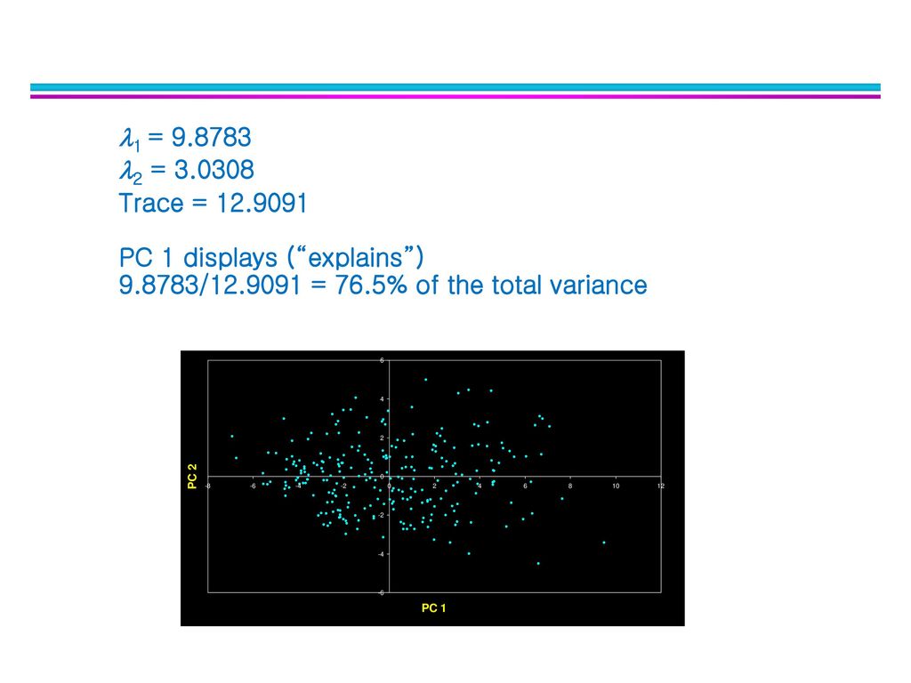
2D Example of PCA Variables X1 and X2 have positive covariance & each has a similar variance.

Principal Components are Computed
PC 1 has the highest possible variance (9.88) PC 2 has a variance of 3.03 PC 1 and PC 2 have zero covariance.

The Dissimilarity Measure Used in PCA is Euclidean Distance
PCA uses Euclidean Distance calculated from the p variables as the measure of dissimilarity among the n objects PCA derives the best possible k dimensional (k < p) representation of the Euclidean distances among objects.

Generalization to p-dimensions
In practice nobody uses PCA with only 2 variables The algebra for finding principal axes readily generalizes to p variables PC 1 is the direction of maximum variance in the p- dimensional cloud of points PC 2 is in the direction of the next highest variance, subject to the constraint that it has zero covariance with PC 1.

PC3 is in the direction of the next highest variance, subject to the constraint that it has zero covariance with both PC1 and PC2 and so on... up to PC p

PC axes are a rigid rotation of the original variables
PC 1 is simultaneously the direction of maximum variance and a least-squares “line of best fit” (squared distances of points away from PC 1 are minimized). PC 1 PC 2 PC1’

if we take the first k principal components, they define the k- dimensional “hyperplane of best fit” to the point cloud of the total variance of all p variables: PCs 1 to k represent the maximum possible proportion of that variance that can be displayed in k dimensions i.e. the squared Euclidean distances among points calculated from their coordinates on PCs 1 to k are the best possible representation of their squared Euclidean distances in the full p dimensions. PC 1 PC 2 PC2’ PC1’

Basic Idea of Feature Reduction Principal Component Analysis Geometric Rationale of PCA The Algebra of PCA Nonlinear PCA using Kernels

Covariance vs Correlation
Using covariances among variables only makes sense if they are measured in the same units even then, variables with high variances will dominate the principal components these problems are generally avoided by standardizing each variable to unit variance and zero mean. Mean variable i Standard deviation of variable i 29 29

Covariance vs Correlation
covariances between the standardized variables are correlations after standardization, each variable has a variance of 1.000 correlations can be also calculated from the variances and covariances: Covariance of variables i and j Correlation Variance of variable j 30 30

The Algebra of PCA first step is to calculate the cross-products matrix of variances and covariances (or correlations) among every pair of the p variables square, symmetric matrix diagonals are the variances, off-diagonals are the covariances. Variance-covariance Matrix Correlation Matrix X1 X2 6.6707 3.4170 6.2384 X1 X2 1.0000 0.5297

So PCA gives New variables zi that are linear combination of the original variables (xi): zi = ai1x1 + ai2x2 + … aipxp ; i = 1..p The new variables zi are derived in decreasing order of importance; they are called ‘principal components’ Example) Sample data variance

The Algebra of PCA in matrix notation, this is computed as
where X is the n x p data matrix, with each variable centered (also standardized by SD if using correlations). Variance-covariance Matrix Correlation Matrix X1 X2 6.6707 3.4170 6.2384 X1 X2 1.0000 0.5297

The Algebra of PCA sum of the diagonals of the variance-covariance matrix is called the trace it represents the total variance in the data it is the mean squared Euclidean distance between each object and the centroid in p-dimensional space. Trace = Trace = X1 X2 6.6707 3.4170 6.2384 X1 X2 1.0000 0.5297 Variance-covariance Matrix Correlation Matrix

The Algebra of PCA finding the principal axes involves eigenanalysis of the cross-products matrix (S) the eigenvalues (latent roots) of S are solutions () to the characteristic equation 35 35

The Algebra of PCA 1 = 9.8783 2 = 3.0308 Note: 1+2 =12.9091
the eigenvalues, 1, 2, ... p are the variances of the coordinates on each principal component axis the sum of all p eigenvalues equals the trace of S (the sum of the variances of the original variables). X1 X2 6.6707 3.4170 6.2384 1 = 2 = Note: 1+2 = Trace =

The Algebra of PCA each eigenvector consists of p values which represent the “contribution” of each variable to the principal component axis eigenvectors are uncorrelated (orthogonal) their cross-products are zero. Eigenvectors a1 a2 X1 0.7291 X2 0.6844 0.7291*( ) * = 0

The Algebra of PCA coordinates of each object i on the kth principal axis, known as the scores on PC k, are computed as where Z is the n x k matrix of PC scores, X is the n x p centered data matrix, A is the p x k matrix of eigenvectors. 38 38

The Algebra of PCA variance of the scores on each PC axis is equal to the corresponding eigenvalue for that axis the eigenvalue represents the variance displayed (“explained” or “extracted”) by the kth axis the sum of the first k eigenvalues is the variance explained by the k-dimensional ordination. 39 39

PCA Eigenvalues λ2 λ1 λ1 = Var(Z1) λ2 = Var(Z2)

λ1 = Var(Z1) λ2 = Var(Z2) The Algebra of PCA
The cross-products matrix computed among the p principal axes has a simple form: all off-diagonal values are zero (the principal axes are uncorrelated) the diagonal values are the eigenvalues. λ1 = Var(Z1) λ2 = Var(Z2) PC1 PC2 9.8783 0.0000 3.0308 Variance-covariance Matrix of the PC axes 41 41

1 = 2 = Trace = PC 1 displays (“explains”) / = 76.5% of the total variance 42 42

Dimensionality Reduction (1/2)
Can ignore the components of less significance. You do lose some information, but if the eigenvalues are small, you don’t lose much n dimensions in original data calculate n eigenvectors and eigenvalues choose only the first p eigenvectors, based on their eigenvalues final data set has only p dimensions

Algebraic derivation of PCs
To find first note that where covariance is the covariance matrix. In the following, we assume the Data is centered.

Assume Form the matrix: then Obtain eigenvectors of S by computing the SVD of X:

Basic Idea of Feature Reduction Principal Component Analysis Geometric Rationale of PCA The Algebra of PCA PCA Algorithm Eigenvector, eigenvalue Nonlinear PCA using Kernels

Find a the best axis !! 투영된 점의 평균과 분산 Max Var[Zi] Subject to aTa= 1 조건부 최적화 문제로 다시 쓰면, L은 라그랑제 함수, λ는 라그랑제 승수 Find a the best axis

미분하고 수식 정리하면, 0으로 놓고 풀면, Train data의 공분산 행렬 S를 구하고, 그것의 a eigenvector 를 구하면 그것이 바로 최대 분산을 갖는 a가 됨

Review Eigenvector Eigenvalue

Definition a is said to be an eigenvector of S corresponding to λ.
A is an n×n matrix, a≠ 0 vector, a ∈ Rn is called an eigenvector of S if Sa is a scalar multiple of a; for some scalar λ. The scalar λ is called an eigenvalue of S, and a is said to be an eigenvector of S corresponding to λ. eigenvector eigenvalue

Example 1: Eigenvector of a 2×2 Matrix
The vector is an eigenvector of Corresponding to the eigenvalue λ=3, since 51 51

PCA Toy Example Consider the following 3D points
If each component is stored in a byte, we need 18 = 3 x 6 bytes

PCA Toy Example Looking closer, we can see that all the points are related geometrically: they are all the same point, scaled by a factor:

PCA Toy Example They can be stored using only 9 bytes (50% savings!):
Store one point (3 bytes) + the multiplying constants (6 bytes)

To find the eigenvalues of an n×n matrix S we rewrite Sa = λa as
Sa = λIa or (S - λI) a = 0 For λ to be an eigenvalue, there must be a≠ 0 if and only if (S - λI)a = 0  | S – λI | = det (S - λI) = 0 This is called the characteristic equation of S; the scalar satisfying this equation are the eigenvalues of S. When expanded, the determinant det (λI-S) is a polynomial p in λ called the characteristic polynomial of S. unit matrix S의 Characteristic equation 55 55

Example 2: Eigenvalues of a 3×3 Matrix (1/3)
Find the eigenvalues of Solution. The characteristic polynomial of S is The eigenvalues of S must therefore satisfy the cubic equation

maximizes subject to To find the best coefficient vector that Let λ be a Lagrange multiplier therefore is an eigenvector of S corresponding to the largest eigenvalue

To find the next coefficient vector maximizing subject to: uncorrelated First note that then let λ and ϕ be Lagrange multipliers, and maximize

We find that is also an eigenvector of S whose eigenvalue is the second largest. In general The kth largest eigenvalue of S is the variance of the kth PC. The kth PC retains the kth greatest fraction of the variation in the sample. 60

알고리즘과 응용 예제 최대 분산을 갖는 축 variance Variance

알고리즘과 응용 을 풀면 D 개의 고유 벡터. 고유값이 큰 것 일수록 중요도가 큼
변환 행렬 을 풀면 D 개의 고유 벡터. 고유값이 큰 것 일수록 중요도가 큼 따라서 D 차원을 d 차원으로 줄인다면 고유값이 큰 순으로 d 개의 고유 벡터를 취함. 이들을 주성분이라 부르고 a1, a2, …, ad로 표기함 변환 행렬 A는, 실제 변환은, 62

Principal Component Analysis (Also called the Karhunen-Loeve transform)
Start PCA with data samples 1. Compute the mean 2. Computer the covariance: 3. Compute the eigenvalues λ and eigenvectors a of the matrix 4. Solve 5. Order them by magnitude: 6. PCA reduces the dimension by keeping direction a such that

Interpretation of PCA The new variables (PCs) have a variance equal to their corresponding eigenvalue Var(zi)= i for all i=1…p Small i  small variance  data change little in the direction of component zi The relative variance explained by each PC is given by li / li

How many components to keep?
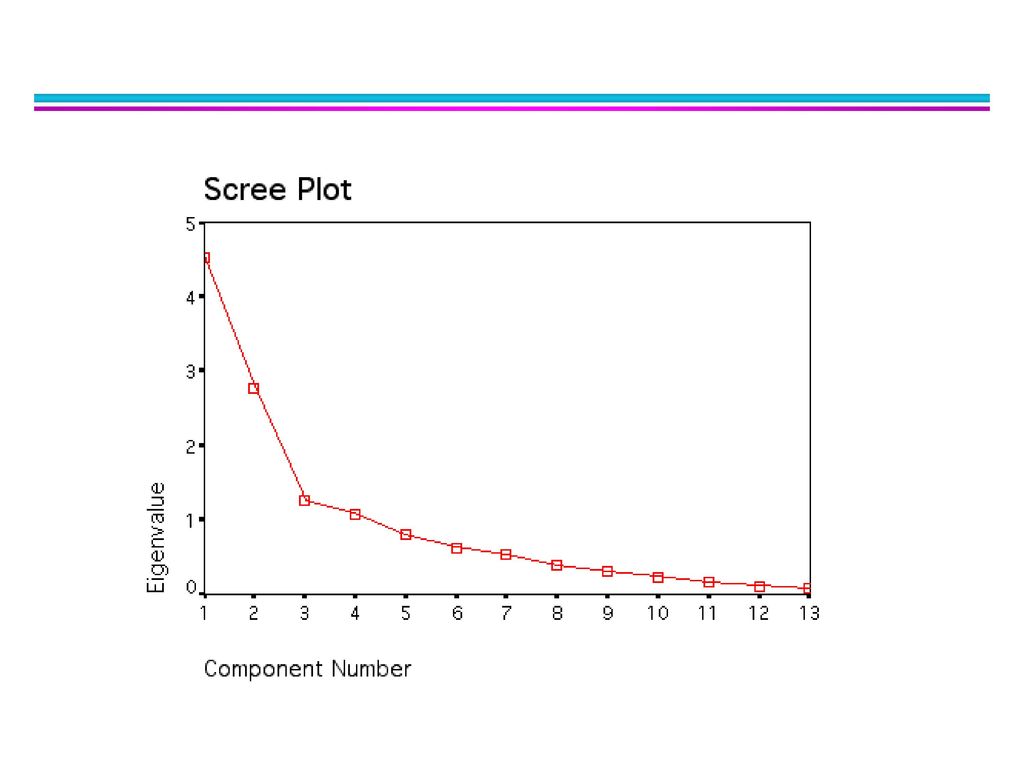
Enough PCs to have a cumulative variance explained by the PCs that is >50-70% Kaiser criterion: keep PCs with eigenvalues >1 Scree plot: represents the ability of PCs to explain de variation in data

Basic Idea of Feature Reduction Principal Component Analysis Geometric Rationale of PCA The Algebra of PCA PCA Algorithm example Nonlinear PCA using Kernels

Principal Component Analysis (Also called the Karhunen-Loeve transform)
Example) * 기호에 주의 !! 68

Karhunen-Loeve 변환(KL-변환), Hotelling 변환
영상의 상관 행렬 변환 !! 영상의 행렬 이진 영상 객체표현 69

70

고유값 계산 Sa = 0 에서 a ≠0 인 해를 얻는 경우는 |S|=0 인 경우다. |S –λI| =0일 때 a ≠0 인 해가 존재한다. : covariance after transformation !!

두 벡타는 각각 Orthogonal, 정규직교에 해당하므로 로 정리할 수 있다.

- 에너지 분포를 고려한 성분분석 (89%가 첫번째 열벡터에 집중) 변환된 자기상관행렬

x의 KL변환은 역 KL변환은

Basic Idea of Feature Reduction Principal Component Analysis Geometric Rationale of PCA The Algebra of PCA PCA Algorithm example Nonlinear PCA using Kernels

Motivation Linear projections will not detect the pattern. 80

Nonlinear PCA using Kernels
Traditional PCA applies linear transformation May not be effective for nonlinear data Solution: apply nonlinear transformation to potentially very high- dimensional space. Computational efficiency: apply the kernel trick. Require PCA can be rewritten in terms of dot product. More on kernels later

Rewrite PCA in terms of dot product The covariance matrix S can be written as Let a be The eigenvector of S corresponding to λ ≠ 0 Eigenvectors of S lie in the space spanned by all data points. 82

The covariance matrix can be written in matrix form: Any benefits?

Next consider the feature space: The (i,j)-th entry of is Apply the kernel trick: K is called the kernel matrix.

Projection of a test point x onto a: Explicit mapping is not required here.

Linear Discriminant Analysis (LDA; 선형판별분석)

Linear Discriminant Analysis (1/6)
What is the goal of LDA? Perform dimensionality reduction “while preserving as much of the class discriminatory information as possible”. Seeks to find directions along which the classes are best separated. Takes into consideration the scatter within-classes but also the scatter between-classes. For example of face recognition, more capable of distinguishing image variation due to identity from variation due to other sources such as illumination and expression.

Covariance: Within-class scatter matrix Between-class scatter matrix projection matrix LDA computes a transformation that maximizes the between-class scatter while minimizing the within-class scatter: products of eigenvalues ! : scatter matrices of the projected data y

Does Sw-1 always exist? If Sw is non-singular, we can obtain a conventional eigenvalue problem by writing: In practice, Sw is often singular since the data are image vectors with large dimensionality while the size of the data set is much smaller (M << N ) c.f. Since Sb has at most rank C-1, the max number of eigenvectors with non-zero eigenvalues is C-1 (i.e., max dimensionality of sub- space is C-1)

Does Sw-1 always exist? – cont. To alleviate this problem, we can use PCA first: PCA is first applied to the data set to reduce its dimensionality. LDA is then applied to find the most discriminative directions:

PCA LDA D. Swets, J. Weng, "Using Discriminant Eigenfeatures for Image Retrieval", IEEE Transactions on Pattern Analysis and Machine Intelligence, vol. 18, no. 8, pp , 1996

Linear Discriminant (선형분별)
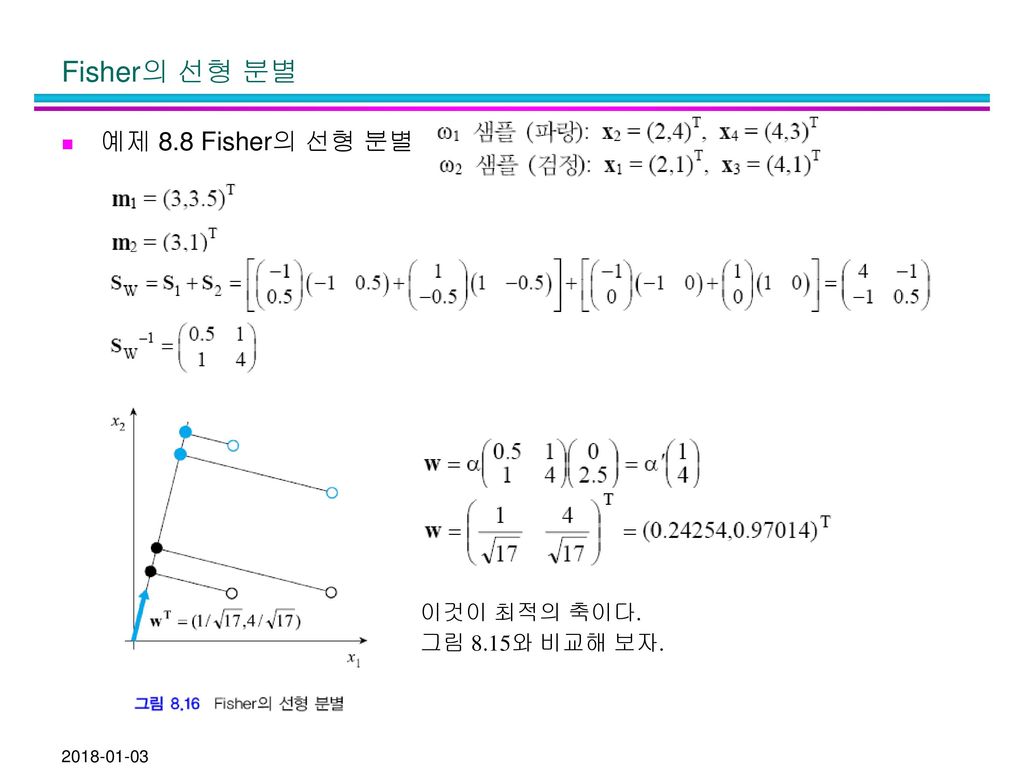
Fisher의 선형 분별 특징 추출이 아니라 분류기 설계에 해당 하지만 PCA와 원리가 비슷함 PCA와 Fisher LD는 목표가 다름 PCA는 정보 손실 최소화 (샘플의 부류 정보 사용 안함) Fisher LD는 분별력을 최대화 (샘플의 부류 정보 사용함) 원리 축으로의 투영 세 개의 축 중에 어느 것이 분별력 관점에서 가장 유리한가? 샘플 x 투영 축 w

Fisher의 선형 분별 문제 공식화 기본 아이디어 유리한 정도를 어떻게 수식 화할까?
가장 유리한 축 (즉 최적의 축)을 어떻게 찾을 것인가? 기본 아이디어 “같은 부류의 샘플은 모여있 고 다른 부류의 샘플은 멀리 떨어져 있을수록 유리하다.” 부류간 퍼짐between-class scatter 부류내 퍼짐within-class scatter

Fisher의 선형 분별 목적 함수 J(w) J(w)를 최대화하는 w를 찾아라. 분자와 분모를 다시 쓰면, 분모 분자

Fisher의 선형 분별 목적 함수를 다시 쓰면, 으로 두고 풀면, (8.49)를 정리하면,
결국 답은 (즉 구하고자 한 최적의 축은),

Fisher의 선형 분별 예제 8.8 Fisher의 선형 분별 이것이 최적의 축이다. 그림 8.15와 비교해 보자.

PCA vs LDA vs ICA PCA : Proper to dimension reduction
LDA : Proper to pattern classification if the number of training samples of each class are large ICA : Proper to blind source separation or classification using ICs when class id of training data is not available

Reference Principal Component Analysis. I.T. Jolliffe.
Kernel Principal Component Analysis. Schölkopf, et al. Geometric Methods for Feature Extraction and Dimensional Reduction. Burges.

Principal Component Analysis

Similar presentations

Presentation on theme: "Principal Component Analysis"— Presentation transcript:

Similar presentations

About project

지원

로그인

Auth with social network:

Principal Component Analysis

Similar presentations

Presentation on theme: "Principal Component Analysis"— Presentation transcript:

Similar presentations

About project

지원