Ch. 12 Forecasting.

Presentation on theme: "Ch. 12 Forecasting."— Presentation transcript:

1 Ch. 12 Forecasting

2 12.1 시계열 분석법 예측법은 크게 두 가지로 분류할 수 있다
정성적(qualitative) 과 정량적(quantitative) 예측법 그 중 정량적 예측법은 다음 두 가지로 분류됨 Time series analysis : 과거 자료의 특징을 이용하여 미래의 자료의 움직임을 예측 Moving average Exponential smoothing Box-Jenkins method (ARIMA method) Causal forecasting (regression analysis) : 자료를 움직이는 주요한 요인을 파악하여 자료의 변동을 표현함. 예측이 주 목적은 아님.

3 Qualitative method

4 Time series analysis

5 Causal method (regression analysis)

6 1) Moving average method
단순평균법의 문제점 즉, 지난 모든 기간의 자료를 예측치 계산에 포함시키는 것을 해결 일정기간보다 오래된 과거자료는 현재자료와 별 관계가 없게 됨 1980 년의 아파트 수요는 내년의 아파트 수요의 예측에 도움이 안됨.

7

8 1-3월 수요의 평균 예제 12.1 2-4월 수요의 평균 39000 30667 33000 33667 34000 34000

9 Choosing an appropriate N and forecast error
In the moving average method, N value is selected to minimize a forecast error. The error is calculated using the previously observed data Several definitions are available for the forecast error Mean of the error Mean absolute deviation Mean squared error

10 Mean absolute deviation
Most widely used for representing the forecast error. Definition MAD for the previous forecast 3기간 예측치에 대한 MAD

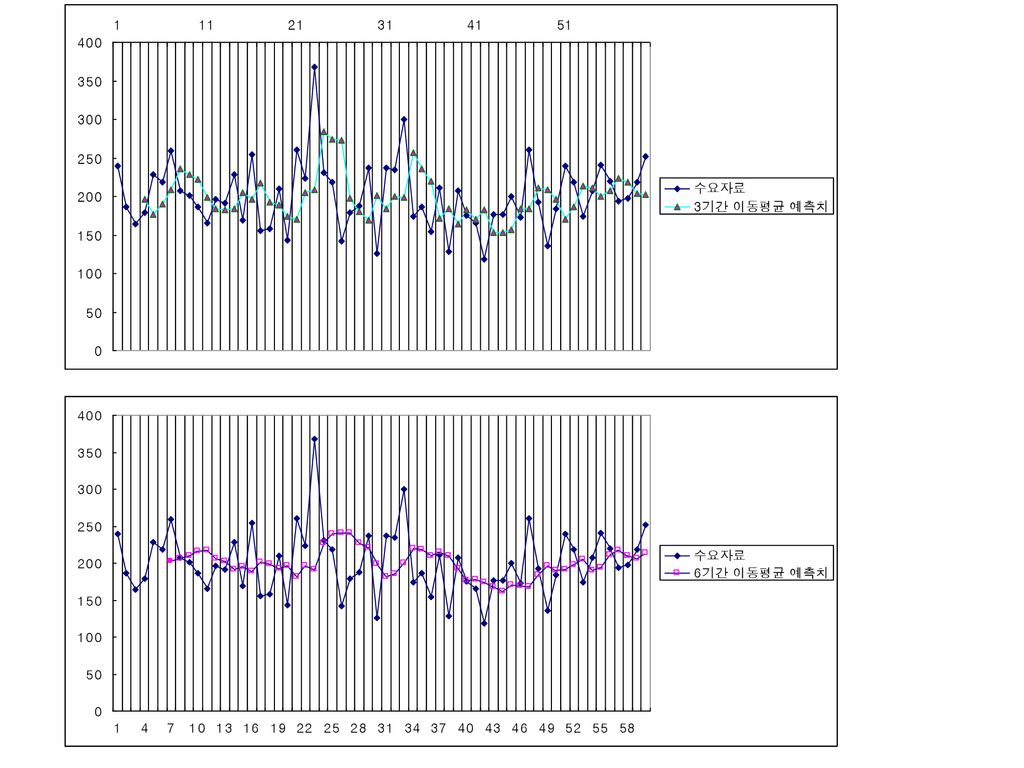
11 Moving average forecasts
Smoother forecast for a larger value of N This is called a smoothing (of the original data) MAD for 3, 6, 20 periods moving average are 41.2, 37.8, 38.3

12

13 Four components of time series
Most of the time series we observe are composed of the following four components Trend – the general direction in which the series is running over a long period Seasonal – relatively short-term repetitive patterns of fluctuations from the trend, usually repeating in year. Cyclical – long-term fluctuation that occur regularly. Difficult to spot. Random – random, irregular or unexpected fluctuations in the series. It is the variation left after removing the above three components.

14 Monthly sales of sweet white wine in Australia
Trend Seasonal Cyclical month Monthly sales of sweet white wine in Australia

15 Exponential smoothing
Frequently used method for demand forecasting Simple and easy Appropriate for a short-term forecasting Enhancing the shortcomings of the moving average A number of variants including Simple exponential smoothing Holt’s method – for time series with trend Winter’s method – for time series with trend and seasonal components

16 Simple exponential smoothing
30000 31638 39000 32374 33000 32437 34000 32593 Simple exponential smoothing Calculate At and use it to forecast Forecast for k period ahead is 로 주어진 것으로 가정함 30000 31800 32000 31820 30000 31638 39000 32374 33000 32437 34000 32593

17 Simple exponential smoothing
어떤 기에 예측되는 미래 모든기간의 예측치는 동일하다. 즉, 7월말에 계산된 8월의 예측치가 300 이라면, 7월말 기준으로 9월 이후의 예측치도 300 이 된다. 그러나 시간이 흘러서 8월말이 되어, 9월의 예측치를 계산하여 320 이 나왔다면 다시 9월 이후의 예측치는 모두 320 이 된다. 즉, 어느 시점 기준으로 모든 미래 시점의 예측치는 동일하며, 다만 시간이 흐름에 따라 미래 시점의 예측치도 바뀌게 된다. 이를 새로운 정보를 이용한다는 관점으로 이해하여야 함.

18 Simple exponential smoothing for one period ahead forecast
Alpha=0.2 의 MAD=35.8, Alpha=0.7 의 MAD=41. Cf. MAD for 3, 6, 20 periods moving average are 41.2, 37.8, 38.3 It is usual to use an alpha value less than 0.3 Alpha higher than 0.3 makes the forecast error bigger.

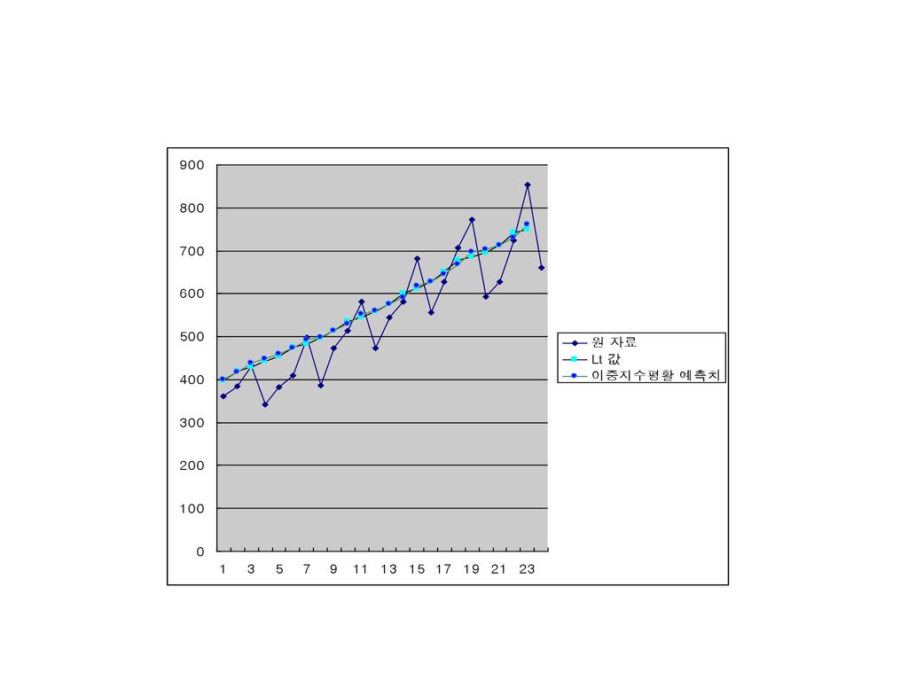
19 Double exponential smoothing (Holt’s method)
Calculate Lt and Tt and use them to forecast Forecast for k period ahead is Lt is base level, Tt is per period trend Lt 는 t 기의 자료의 크기를 나타낸다. Tt 는 t 기의 시계열의 기울기를 나타낸다. t 기의 Lt 의 실측치 t-1 기의 Lt 의 예측치 각각 Tt 의 실측 과 예측치

20

21 Example 12.3 Holt’s method 주어진 값으로 가정해도 무방 Find T0 and L0 L0
가장 최근의 관찰값 L0

22 Example 12.3 Holt’s method When we assume ,we obtain the result in Table 12.3 t 실제 관찰된 수요 Lt Tt ft-1, et 40 37.71 2.83 첫 번째 두 번째 세 번째 40.54 1 월말에 실제 수요치 40 을 관찰하고 Lt 를 계산한다. Lt 를 이용하여 Tt 를 계산한다. ft,1 을 계산한다 (위 경우는 40.54). 한 기간이 진행될 때마다 위의 과정을 반복한다. 네 번째

23 Example 12.3 Holt’s method

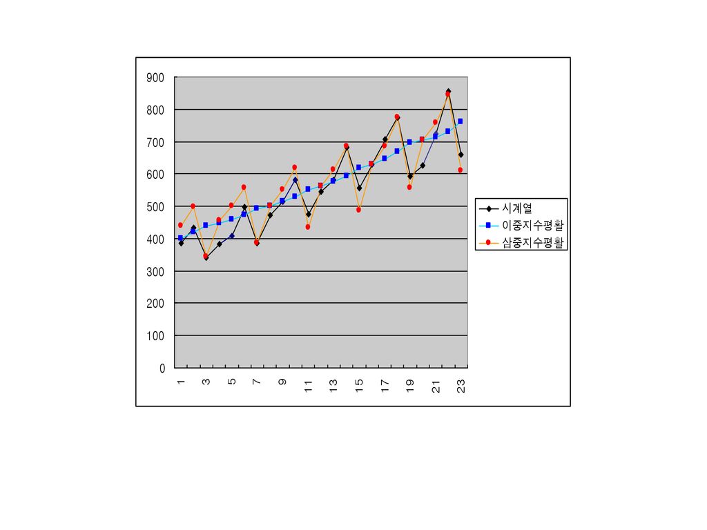
24 Triple exponential smoothing (Winter’s method)
이중지수평활이 계절적 요인을 잘 반영하지 못하는 부분을 보완 세 종류의 값과 세 가지의 식을 이용한다. 이전 식과 유사

25 Triple exponential smoothing (Winter’s method)
C: 계절변동이 나타나는 길이 St: 계절지수 예를 들어 분기별 자료면 c=4, 월간 자료면 c=12 가 된다. 다음 식을 이용하여 Lt , Tt 와 St 를 계산한다. t기의 Lt 의 실측치 t-1 기의 Lt 의 예측치 각각 St 의 실측 과 예측치

26 Forecast for k period ahead is
예측하려는 시점 t+k=18+9=27 가장 최근의 3월 계절지수 예측값의 계산 6월 현재시점, t=18 Forecast for k period ahead is n 은 인 가장 작은 값으로 선택 이것은 가장 최근의 같은 계절의 계절지수를 사용한다는 의미이다. 예를 들어 년간자료 즉, C=12 이고, 현재 시점이 6월 일 때 (t=18 기라고 봄), 내년 3월 (k=9) 에 대한 예측을 하는 경우에는 n=1 로 하여 올해 3월(t+k-C= =15 기) 의 계절지수를 사용한다.

27 Example 12.4 Winter’s method
T0 , L0 와 St 가 다음과 같이 주어졌다. 간략한 설명을 위하여 책과는 달리 주어진 것으로 본다. 계절요인의 값은 다음 슬라이드와 같이 주어짐.

28 Example 12.4 Winter’s method
주어진 St 값 St 는 다음 표의 가장 오른쪽 열과 같이 주어졌다. 월 수요/ 94 년 평균 월 수요/95 년 평균

29 Example 12.4 Winter’s method
다섯 번째 Example 12.4 Winter’s method We obtain the result in Table 12.5 t 실제 관찰된 수요 Lt Tt St ft-1,1 13 53.17 3.87 0.23 첫 번째 두 번째 세 번째 네 번째 9.13 1 월말에 실제 수요치 13 을 관찰하고 Lt 를 계산한다. Lt 를 이용하여 Tt 를 계산한다. Tt 를 이용하여 St 를 계산하고 모든 계절지수를 정규화한다. ft,1 을 계산한다 위의 과정을 반복한다.

30 Example 12.4 Winter’s method (Excel)

31 계절지수의 정규화 이 예제에서는 12.01 로 0.01 의 오차만 생겨서 정규화 한 후의 값이 변하지 않았다.
When we calculate a new St, we have to normalize the whole St values to make them sum to C (cyclical length). Example of the normalization(428쪽 참조) 1월말 정규화된계절지수 초기계절지수 1월말 계절지수 각 St 값에 (12/12.01) 을 곱하여 이 예제에서는 로 0.01 의 오차만 생겨서 정규화 한 후의 값이 변하지 않았다.

32 계절지수 (Excel 활용

33