Neural Network 의 변천사를 통해 바라본 R 에서 Deep Neural Network 활용 Produced by Tae Young Lee.

Presentation on theme: "Neural Network 의 변천사를 통해 바라본 R 에서 Deep Neural Network 활용 Produced by Tae Young Lee."— Presentation transcript:

1 Neural Network 의 변천사를 통해 바라본 R 에서 Deep Neural Network 활용 Produced by Tae Young Lee

2 이반 페트로비치 파블로프 (Иван Петрович Павлов, 1849 년 1849 년 9 월 26 일 - 1936 년 2 월 27 일 ) 는 러시아의 생리학자9 월 26 일1936 년2 월 27 일 러시아 생리학 생물심리 전자회로 의학 컴퓨터공학

3

4

5

6

7 Formula

8 인지 학습 추론 강화

9 출처 : http://blog.revolutionanalytics.com/2013/06/a-list-of-r-packages-by- popularity.html

10

11

12

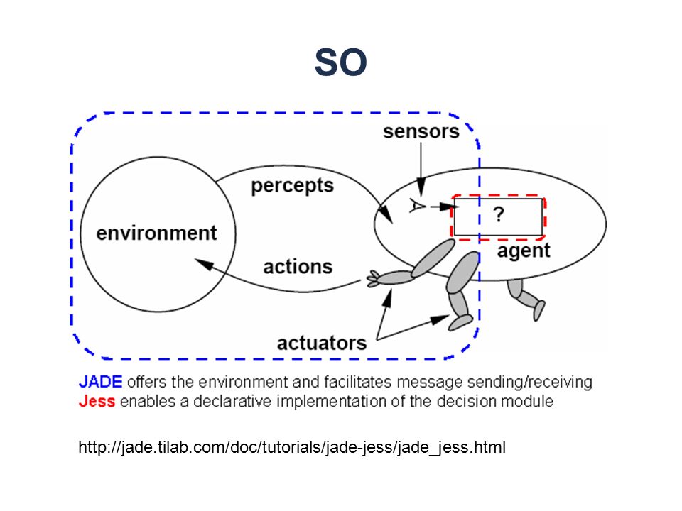
13 http://jade.tilab.com/doc/tutorials/jade-jess/jade_jess.html

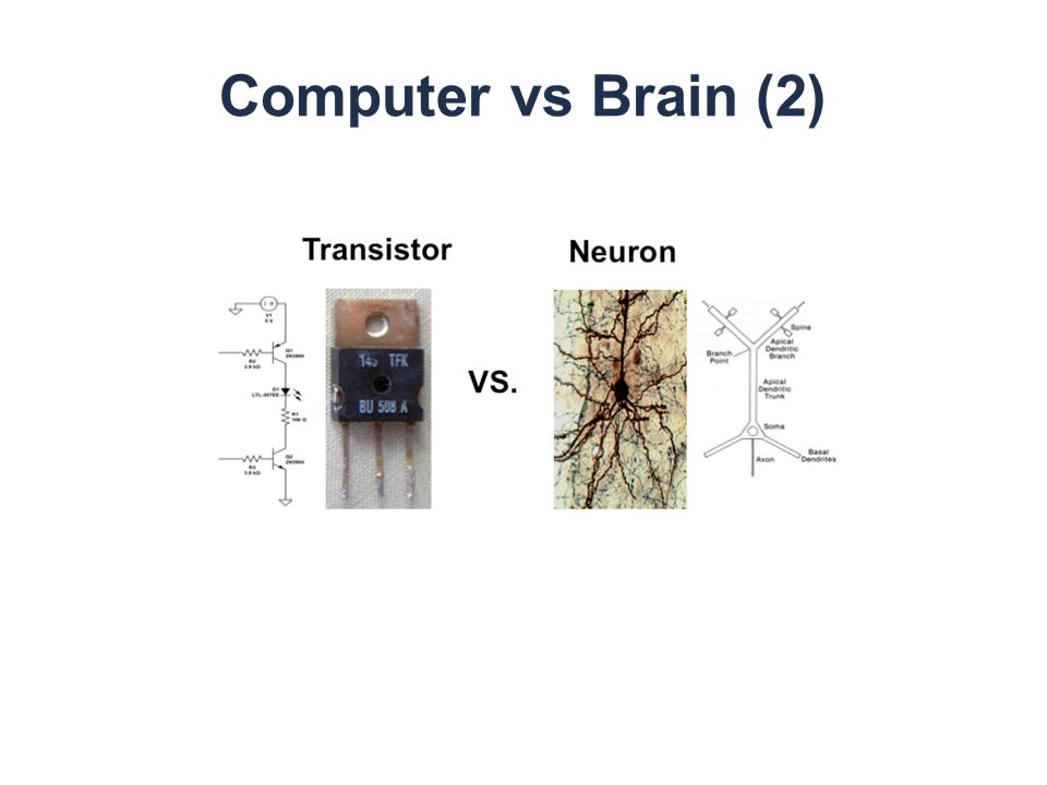
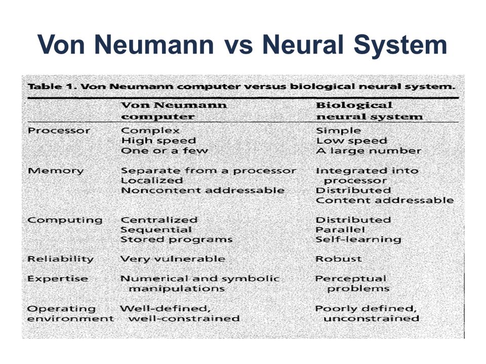
14 100 억개의 neurons 60 조의 synapses Distributed Processing Non linear Processing Parallel Processing Central Processing Arithmetic operation’ (linearity) Sequential Processing

15

16 제 1 신경망은 알렉산더 베인 (1818 - 1903) 에 의해 제시되었다. "Mind and Body The Theories of Their Relation". 1873 년 Bain's Summation Threshold Network Bain's Signal Attenuation Proposal Restatement of Bain's Adaptive Rule by William James (1890) 1890 년

17 Signal Attenuation( 신호 감쇠 ) Threshold( 임계값 )

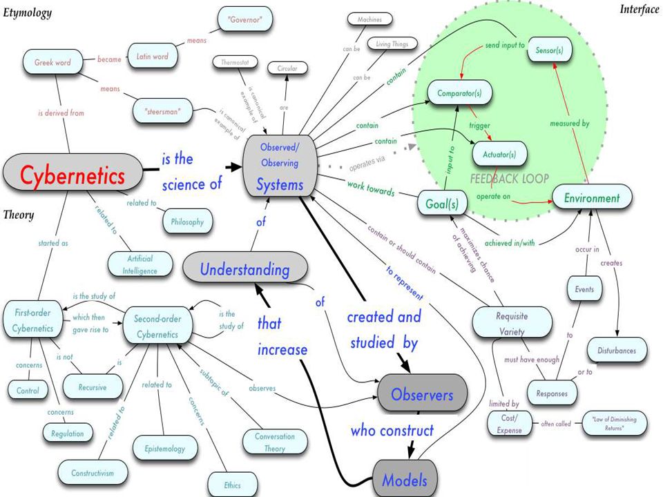
18 고전적 조건화의 행동적 연구 ( 파블로프의 개 ) CYBERNETICS

19 사이버네틱스 또는 인공두뇌학은 일반적으로 생명체, 기계, 조직과 또 이들의 조합 을 통해 통신과 제어를 연구하는 학문이다. 예를 들어, 사회 - 기술 체계에서 사이버네 틱스는 오토마타와 로봇과 같은 컴퓨터로 제어된 기계에 대한 연구를 포함한다. 생명체 기계 조직 통신 제어 사회 - 기술 체계 오토마타 로봇 사이버네틱스라는 용어는 고대 그리스어 퀴베르네테스 Κυβερνήτης (kybernetes, 키 잡이, 조절기 (governor), 또는 방향타 ) 에서 기원한다. 고대 그리스어 Κυβερνήτης 예로부터 현재까지 이 용어는 적응계, 인공지능, 복잡계, 복잡성 이론, 제어계, 결정 지지 체계, 동역학계, 정보 이론, 학습 조직, 수학 체계 이론, 동작연구 (operations research), 시뮬레이션, 시스템 공학으로 점점 세분화되는 분야들을 통칭하는 용어 로 쓰이고 있다. 적응계 인공지능 복잡계 복잡성 이론 제어계 결정 지지 체계 동역학계 정보 이론 학습 조직 수학 체계 이론 동작연구 시뮬레이션 시스템 공학

20

21 1943 년 neurophysiologist Warren McCulloch mathematician Walter Pitts how neurons might work( 논문 ) Dendrites ( 수상돌기 ) Cell body Nucleus Axon hillock ( 축색둔덕 ) Axon ( 축색 ) Signal direction Synapse ( 시냅스 ) Myelin sheath Synaptic terminals Presynaptic cell ( 시냅스전 신경세포 ) Postsynaptic cell ( 시냅스후 신경세포 ) Synaptic terminal ( 시냅스 말단 ) 뇌의 신경 세포가 작동 할지도 모른다 방법을 설명하기 위해, 그들은 전기 회로를 사용한 간단한 신경망 모델링하였다.

22 1949 년 Donald Hebb The Organization of Behavior( 논문 ) LTP(Long Term Potential) : 장기 강화

23 Symbolic AI

24 모든 지능형 생각이 symbolic 조작이라는 가설.

25 1954 년 The First Randomly Connected Reverberatory Networks The Farley and Clark Network Hebbian 영감 네트워크는 MIT 의 최초의 디지털 컴퓨터에서 1954 년에 팔리와 클 라크에 의해 시뮬레이션했습니다. 네트워크는 무작위로 곱셈 계수 ( 가중치 ) 를 갖는 단방향 선으로 서로 연결 뉴런을 나타내는 노드로 구성됩니다. multiplication factors (weights).

26 1956 년 The First Reverbatory Network Showing Self-Assembly One Cell of the Self-Assembly Network Poughkeepsie, New York 에있는 IBM 연구소의 초기 IBM 유형 701 (2K 바이트의 메모리 ) 및 704 계산기를 사용하여 N. 로체스터 과 친구들에 의해 1956 년에 촬영 되었습니다. 전체를 무작위로 셀로 연결하는 것 대신에 Farley and Clark 그들이 단일 층에 세포 를 조직 한 후 무작위로 셀의 출력은 다른 백 셀의 입력에 연결되었습니다

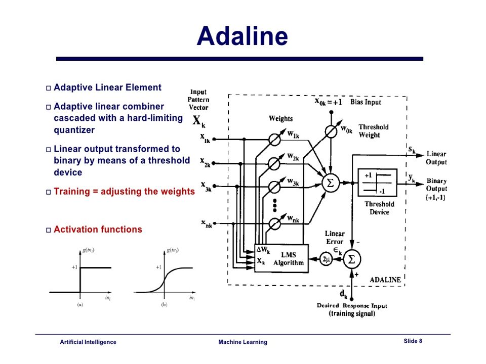
27 1959 년 [Stanford] Bernard Widrow Marcian Hoff developed models called "ADALINE" and "MADALINE.“ Multiple ADAptive LINear Elements

28

29 100 억개의 neurons 60 조의 synapses Distributed Processing Non linear Processing Parallel Processing Central Processing Arithmetic operation’ (linearity) Sequential Processing

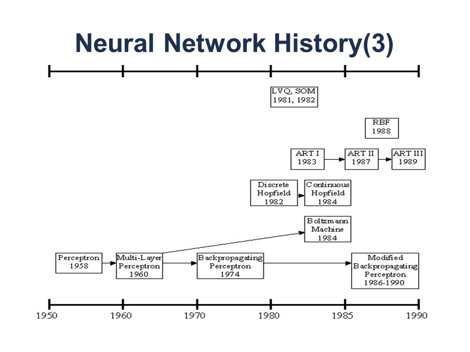
30 1960 년 최초의 artificial neural network 가 연구되기 시작하였다. 이 때는 input, output 의 두 개의 layer 를 사용하였고, 각 layer 의 neuron 과 neuron 을 잇는 synapse 의 weight 를 학습시켜서 물체 인식을 하는 연구가 진행되었다. 이 때는 training data 를 통해서 weight 를 자동으로 학습할 수는 없었고, 사람이 수동으로 튜닝을 해야 만 했다. 이러한 구조는 XOR 문제를 풀 수 없다는 근원적인 단점을 가지고 있었 다. 배타적 논리합 (exclusive or) 은 수리 논리학에서 주어진 2 개의 명제 가운데 1 개 만 참일 경우를 판단하는 논리 연산이다. 약칭으로 XOR, EOR, EXOR 라고도 쓴 다. 수리 논리학 논리 연산

31 1962 년 1962 년에는 Widrow & Hoff 무게는 그것을 조정하기 전에 값을 조사 학습 방법을 개발했다 ( 즉, 0 또는 1) 에 따 라 : 체중 변화 = ( 미리 무게 라인 값 ) * ( 오류 / ( 입력 수 )). 이것은 하나의 활성 퍼셉 트론은 큰 오차를 가지고 있어도 좋지만, 하나의 네트워크를 통해, 또는 적어도 인 접 퍼셉트론에 배포하는 가중치를 조정할 수 있다는 생각에 기초하고 있습니다. 무게의 이전 행이 0 이면, 이것은 궁극적으로 자동으로 수정됩니다 만, 이 규칙을 적용하면 여전히 오류가 발생합니다. 그것이 모든 오류보다 가중치 모두에 전달 되도록 오류가 저장되어있는 경우 제거됩니다.. 아이러니하게도, 존 폰 노이만 자신이 전신 릴레이 나 진공관을 사용하여 신경 기 능의 모방을 시사했습니다. 이것은 여러 신경망의 초기 성공은 특히 시간에 실용적인 기술을 고려하여 신경 망의 가능성을 과장으로 이어졌다는 사실과 결합 시켰습니다. The Classic Perceptrons

32

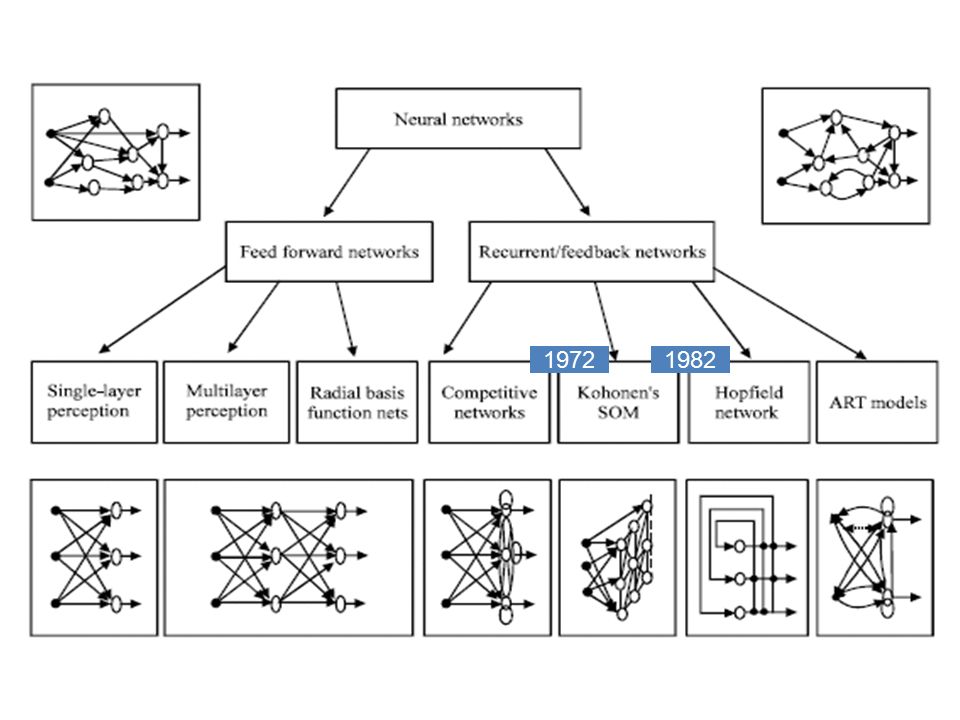
33 1972 년 서로 독립적으로 동일한 네트워크를 개발했습니다. 그들은 모두 자신의 생각을 설 명하기 위해 매트릭스 수학을 사용하지만, 그들은 아날로그 ADALINE 회로의 배열을 만들고 있었지만 현실화 되지는 못하였습니다. 뉴런은 대신 하나 뿐인 출력 세트를 활성화합니다. An Association Network The Association Networks of Kohonen and Anderson

34 1975 년 The first multilayered network was developed in 1975, an unsupervised network. The Repeatable Unit of the Cognitron The Cognitron - First Multilayered Network The NeoCognitron's Position Independence Strategy

35 부장님 출근 하셨나요 ? 차가 주차장에 있었어요

36 ConnectionismNeural Net(ML)

37 파란선과 빨간선의 영역을 구분한다고 생각해보자. 그냥 구분 선을 긋는다 면 아마 왼쪽처럼 불완전하게 그을 수 있을 것이다. 하지만 공간을 왜곡하면 오른쪽 같이 아름답게 구분선을 그릴 수 있다. 이처럼 인공신경망은 선 긋고, 구기고, 합하고를 반복하여 데이터를 처리한다. ( 사진출처 : colah's blog)colah's blog

38 19821972

39 1982 년 John Hopfield of Caltech the National Academy of Sciences 그의 접근 방식은 양방향 라인을 사용 하여 더 유용한 시스템을 만드는 것이 었습니다. 이전 뉴런 간의 연결은 단지 하나임 The Hopfield Association Network – Revival of the Reverberatory Networks Hopfield Network Examples Reilly and Cooper used a "Hybrid network" with multiple layers, each layer using a different problem-solving strategy. Two Layer Hybrid Network

40 1985 년 perceptron 들에 기반한 여러 개의 hidden layer 를 갖는 neural network 가 Geoffrey Hinton 에 의해서 개발되기 시작하였다. Geoffrey E. Hinton 은 현재 Deep learning 의 대가로 알려져 있다. 비슷한 시기에 Geoffrey E. Hinton 은 Boltzmann machine 에 대한 연구로 현재 Deep learning 이 Restricted Boltzmann machine 을 사용한다는 것을 고려할 때 이미 30 년 전부터 초석을 다져왔다고 볼 수 있다. 현재 Geoffrey E. Hinton 은 Yoshua Bengio 과 함께 Deep learning 의 선구자로 알 려져 있다. 이러한 multi-layer perceptron (MLP) 는 글자 인식 등에 널리 사용되었지만 supervised learning 알고리즘이므로 unlabeled data 를 처리할 수 없고, learning 속도가 너무 느리다는 단점이 있다. 또한 learning 이 gradient 기반 방식이므로 initial state 에 크게 영향을 받고, local optima 에 빠진다는 단점이 있다.

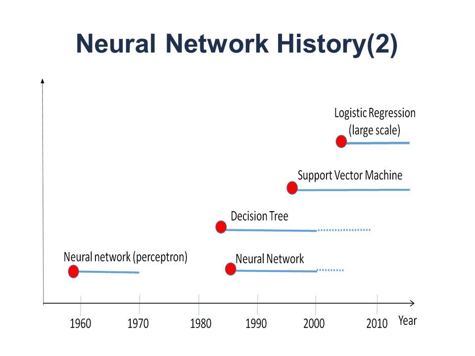
41 1995 년 Vladimir N. Vapnik 과 연구자들이 support vector machine (SVM) 을 처음 제안하였 다. SVM 은 kernel function 을 통해서 input data 를 다른 높은 차원의 공간으로 mapping 을 하고, 이 공간에서 classification 을 하는 구조를 갖고 있다. 이러한 간단 한 구조덕분에 SVM 은 빠른 시간에 학습이 가능하고, 여러 실제적인 문제에 잘 적 용이 되었다. 하지만 shallow architecture 를 갖고 있다는 측면에서 SVM 은 AI 에 있 어서 좋은 연구 방향은 아니라고 평가 받는다. AI 측면에서 긍정적인 구조는 다음의 측면을 가져야 한다고 제안한다. 1) input data 를 통해서 prior knowledge 를 학습할 수 있어야 한다. 2) 여러 개의 layer 를 갖는 구조여야 한다. 3) 여러 개의 학습 가능한 parameter 를 갖고 있어야 한다. 4) 확장 가능해야 한다. 5) Supervised learning 만이 아니라 multi-task learning, semi-supervised learning 등의 학습도 가능해야 한다. 위의 다섯 가지 특성은 Deep learning 이 다른 구조 (MLP, SVM 등 ) 들과 다른 특성 이다. 예를 들면 MLP 는 supervised learning 만이 가능하고, SVM 은 하나의 layer 를 갖는 shallow architecture 이다. 기본적으로 Deep learning 은 여러 개의 layer 를 갖는 구조를 지칭하므로 수 많은 구조가 가능 할 수 있다. 하지만 그 중에서도 Deep Belief Network (DBN) 이 가장 큰 milestone 이라고 할 수 있다.

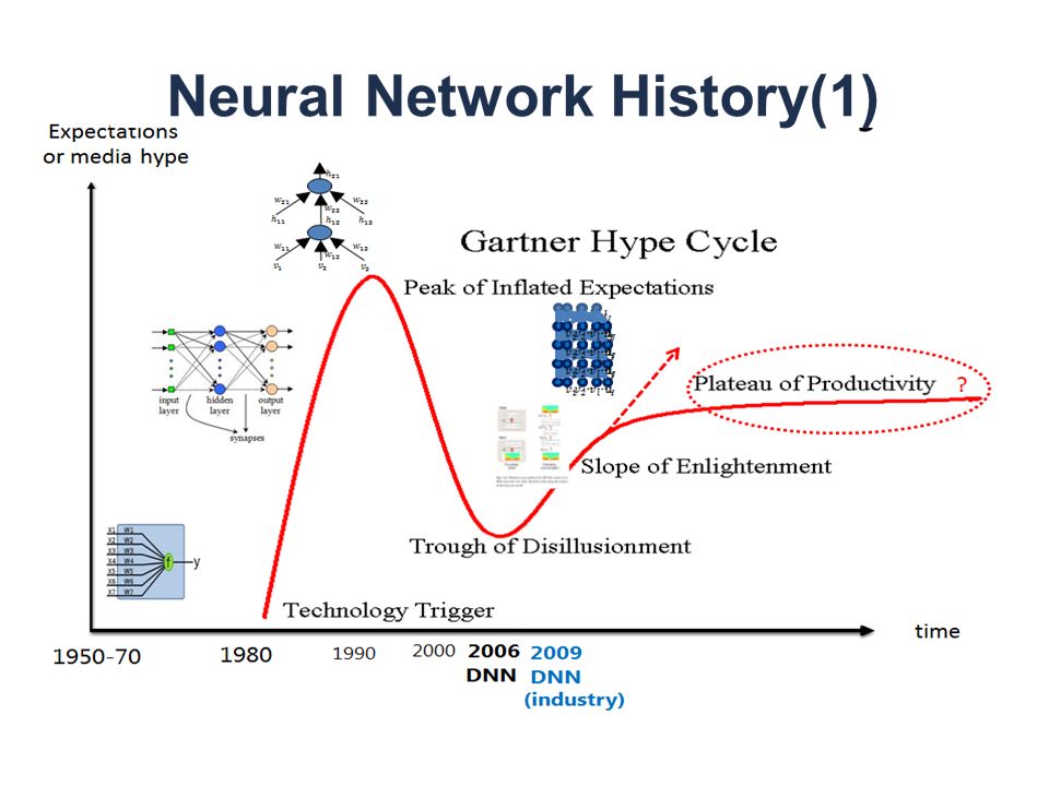
42 2006 년 Geoffrey E. Hinton 은 Deep Belief Network (DBN) 이라는 구조를 제안하였다. DBN 은 기존의 fully connected Boltzmann machine 을 변형하여 layer 와 layer 사이에만 connection 이 있는 restricted Boltzmann machine 을 사용하여서 학습을 좀 더 용이 하게 하였다. 또한 기존의 back-propagation 방법이 아닌 Gibbs sampling 을 이용한 contrastive divergence (CD) 방식을 사용해서 maximum likelihood estimation (MLE) 문제를 풀 었다. 즉 training data 에서 input 과 output 이 필요한 것이 아니기 때문에 unsupervised learning 과 semi-supervised learning 에 적용할 수 있게 되었다. 또한 최상위 층에 MLP 등을 이용해서 supervised learning 에서 사용될 수 있는 장점이 있다.

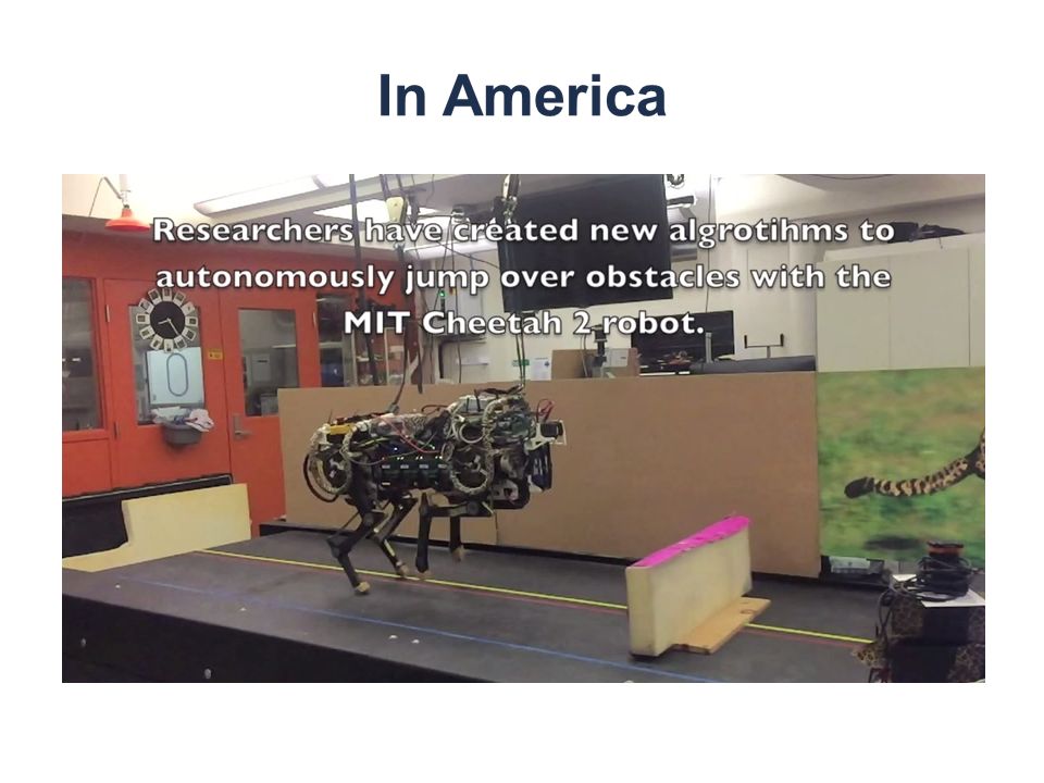
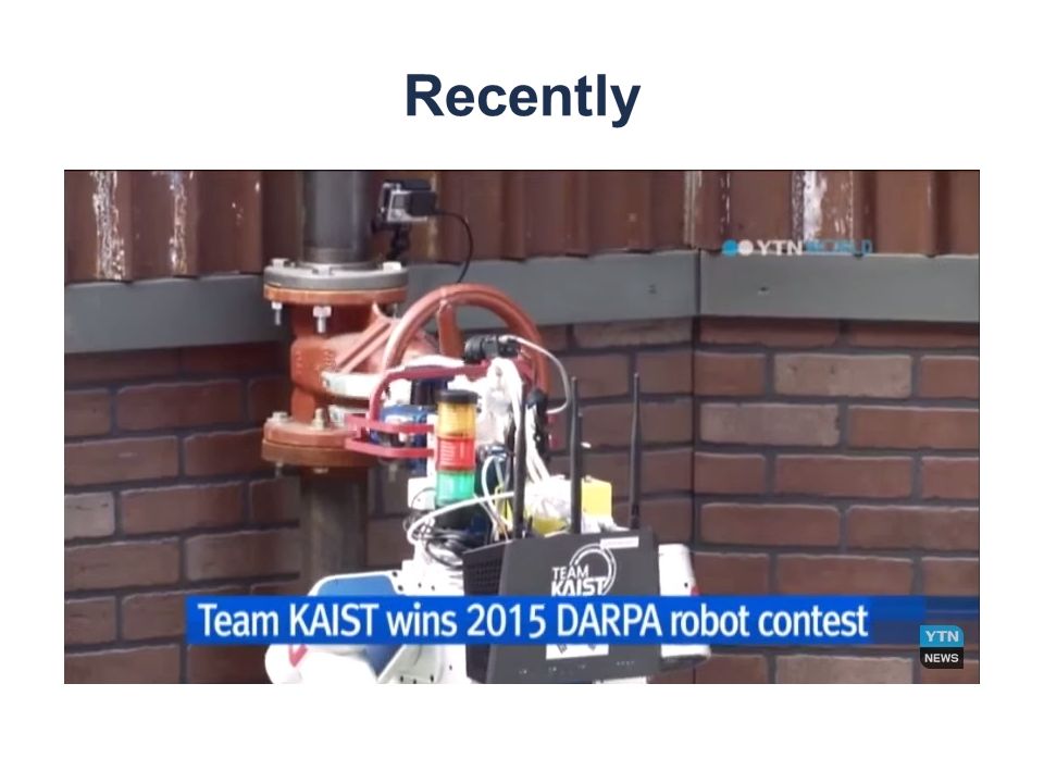
43 Autonomous RobotsAction Science

44

45 library(datasets) names(infert) # | train the network library(neuralnet) nn <- neuralnet( case~age+parity+induced+spontaneous, data=infert, hidden=2, err.fct="ce", linear.output=FALSE) # | output training results # basic nn # reults options names(nn) # result matrix nn$result.matrix out <- cbind(nn$covariate,nn$net.result[[1]]) dimnames(out) <- list(NULL, c("age", "parity","induced","spontaneous","nn-output")) head(out) # generalized weights # The columns refer to the four covariates age (j = # 1), parity (j = 2), induced (j = 3), and spontaneous (j=4) head(nn$generalized.weights[[1]]) # visualization plot(nn)

46 p <- 2 # input space dimension N <- 200 # number of observations set.seed(1) x <- matrix(rnorm(N*p),ncol=p) y 1.4) # In this case, there is a decision boundary # that perfectly separates the data mydata <- data.frame(x=x,y=y) mydata[1:3,] library(nnet) set.seed(3) nn1 <- nnet(y~x.1+x.2,data=mydata,entropy=T,size=3,decay=0,maxit=2000,trace=T) yhat <- as.numeric(predict(nn1,type='class')) par(mfrow=c(1,2)) plot(x,pch=19,col=c('red','blue')[y+1],main='actual labels',asp=1) plot(x,col=c('red','blue')[(yhat>0.5)+1],pch=19,main='predicted labels',asp=1) table(actual=y,predicted=predict(nn1,type='class')) # Re-run the above with seed=4... set.seed(4) nn1 <- nnet(y~x.1+x.2,data=mydata,entropy=T,size=3,decay=0,maxit=2000,trace=T) yhat <- as.numeric(predict(nn1,type='class')) par(mfrow=c(1,2)) plot(x,pch=19,col=c('red','blue')[y+1],main='actual labels',asp=1) plot(x,col=c('red','blue')[(yhat>0.5)+1],pch=19,main='predicted labels',asp=1) par(mfrow=c(2,2)) for (i in 1:4){ set.seed(3) nn1 <- nnet(y~x.1+x.2,data=mydata,entropy=T,size=i,decay=0,maxit=2000,trace=T) yhat <- as.numeric(predict(nn1,type='class')) plot(x,pch=20,col=c('red','blue')[yhat+1],cex=2) title(main=paste('nnet with',i,'hidden units')) }

47 n1 <- 100 n2 <- 110 set.seed(3) nn1 <- nnet(y~x.1+x.2,data=mydata,entropy=T,size=3,decay=0,maxit=2000,trace=T) x1grid <- seq(-3,3,l=n1) x2grid <- seq(-3,3,l=n2) xg <- expand.grid(x1grid,x2grid) xg <- as.matrix(cbind(1,xg)) h1 <- xg%*%matrix(coef(nn1)[1:3],ncol=1) h2 <- xg%*%matrix(coef(nn1)[4:6],ncol=1) h3 <- xg%*%matrix(coef(nn1)[7:9],ncol=1) par(mfrow=c(2,2)) contour(x1grid,x2grid,matrix(h1,n1,n2),levels=0) contour(x1grid,x2grid,matrix(h2,n1,n2),levels=0,add=T) contour(x1grid,x2grid,matrix(h3,n1,n2),levels=0,add=T) title(main='boundaries from linear functions\n in hidden units') sigmoid <- function(x){exp(x)/(1+exp(x))} z <- coef(nn1)[10]+coef(nn1)[11]*sigmoid(h1)+coef(nn1)[12]*sigmoid(h2)+ coef(nn1)[13]*sigmoid(h3) contour(x1grid,x2grid,matrix(z,n1,n2)) title('sum of sigmoids \n of linear functions') contour(x1grid,x2grid,matrix(sigmoid(z),n1,n2),levels=0.5) title('sigmoid of sum of sigmoids \n of linear functions') contour(x1grid,x2grid,matrix(sigmoid(z),n1,n2),levels=0.5) points(x,pch=20,col=c('red','blue')[y+1]) title('data values')

48 library(ggplot2) library(RSNNS) library(MASS) library(caret) head(diamonds) diamonds <- diamonds[sample(1:nrow(diamonds),nrow(diamonds)),] #sample d.index <- sample(0:1, nrow(diamonds),prob=c(0.3,0.7),rep=T) d.train <- diamonds[d.index==1, c(-5,-6)] d.test <- diamonds[d.index==0, c(-5,-6)] dim(d.train) dim(d.test) # linear regression with CV 10 #### # train regression ds.lm <- caret::train(d.train[,-5], d.train[,5], method="lm", trainControl=trainControl(method="cv")) ds.lm #compare observed and predicted train prices ggplot(data.frame(obs=d.train[,5], pred=ds.lm$finalModel$fitted.values),aes(x=obs,y=pred))+geom _point(alpha=0.1)+geom_abline(color="blue")+labs(title="Diamon d Train Prices",x="observed",y="predicted")

49

50