확률현상의 관찰과 실험 아주대학교 이승호 031-219-2560

Presentation on theme: "확률현상의 관찰과 실험 아주대학교 이승호 031-219-2560"— Presentation transcript:

1 확률현상의 관찰과 실험 아주대학교 이승호 031-219-2560 sholee@ajou.ac.kr

2 X( ) 확률변수 1, 3, 5, 2, 4, 6, 를 던지면 ==> 무엇이 나올 지 모른다 (?)  나올 수 있는 것들을 다 적어보자 표본공간

3 3, 2, 6, 1, 2, 3, 5,... ? 02136457 실험 : 를 실제로 굴려 무엇이 나오는 지 관찰하자 X 확률변수 실현 값 관측 값 X 확률변수 실현 값 관측 값

4 3, 2, 6, 1, 2, 2, 5, ? 02136457 실험 : 를 계속 굴려보면 각 값들이 어떻게 나올까 ? ?

5 124365 1/6 ???

6 (1, 3) => 2.0 (6, 2) => 4.0 (2, 5) => 3.5

7 124365 1/6 ???

8 DISCRETE PROBABILITY DISTRIBUTIONS The Binomial Distribution The Geometric and Negative Binomial Distributions The Hypergeometric Distribution The Poisson Distribution The Multinomial Distribution

9 Probability mass function and cumulative distribution function of a B (8, 0.5) random variable

10 Probability mass function and cumulative distribution function of a B (8, 1/3) random variable

11 Probability mass function and cumulative distribution function of a B (8, 0.5) random variable

12 CONTINUOUS PROBABILITY DISTRIBUTIONS 1 The Uniform Distribution 2 The Exponential Distribution 3 The Gamma Distribution 4 The Weibull Distribution 5 The Beta Distribution

13 Probability density function of a U(a, b) distribution Probability density function of a U(a, b) distribution

14 Probability density function of an exponential distribution with parameter = 1

15 Probability density functions of gamma distributions

16 Probability density functions of the Weibull distribution Probability density functions of the Weibull distribution

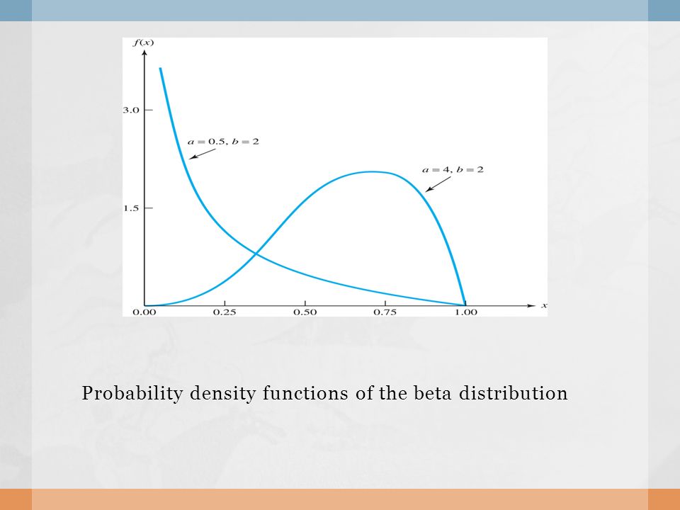
17 Probability density functions of the beta distribution

18

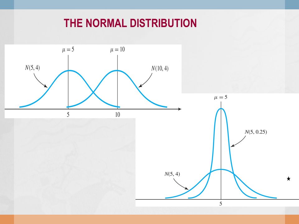
19 The standard normal distribution THE NORMAL DISTRIBUTION

20

21 대수의 법칙 Law of Large Numbers Borel 의 대수의 법칙 => Kolmogorof 의 대수의 법칙 =>

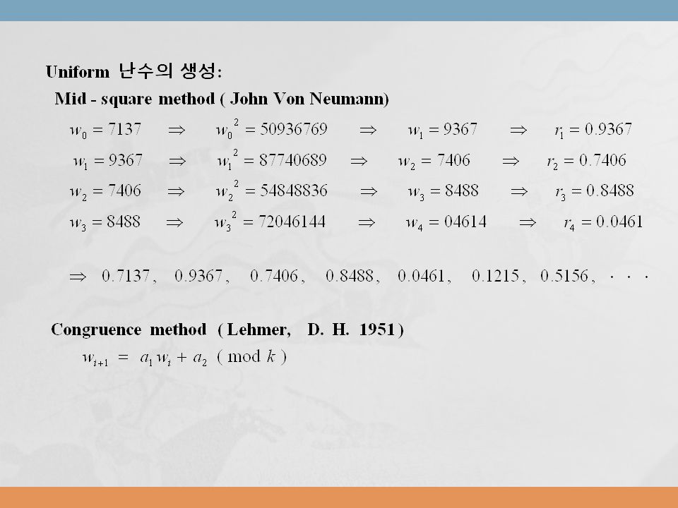
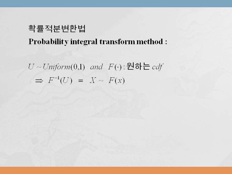
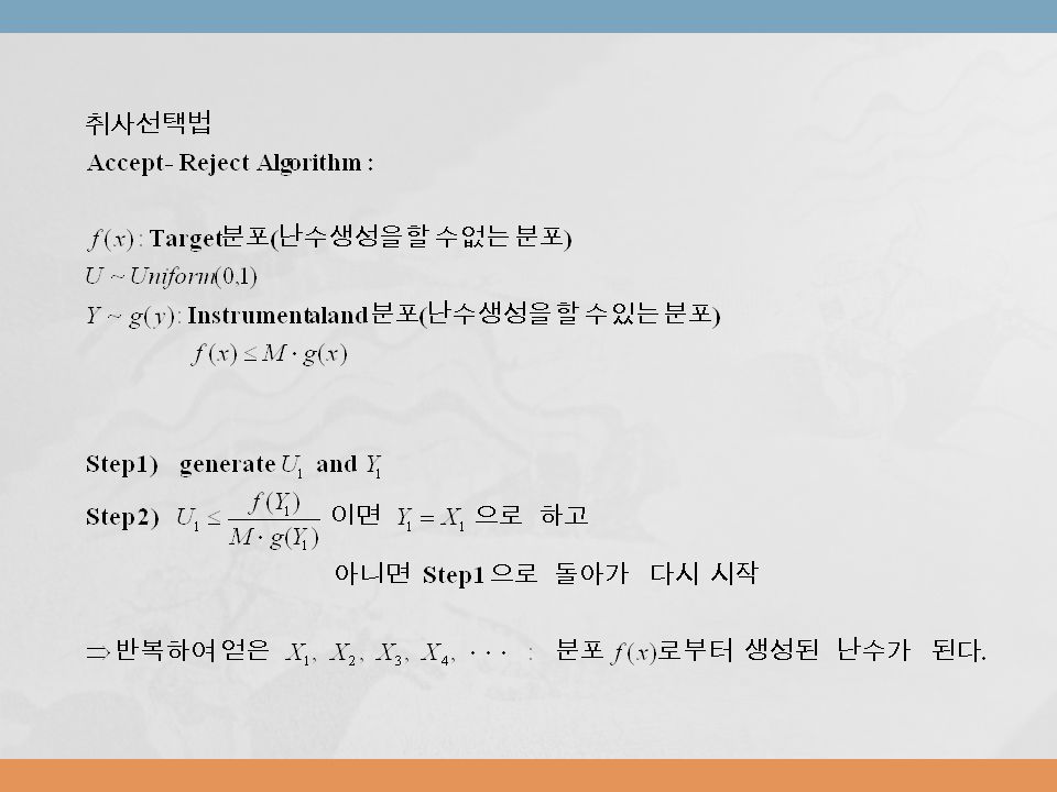
22 Generation of Pseudo-Random Numbers The Standard Uniform Distribution ( mid-square method, congruence method) The Integral Transform Methods ( Exponential Distribution, etc. ) The Accept-Reject Methods ( Gamma Distribution, The Weibull Distribution)

23

24

25

26 안과 밖에서 접하는 정다각형으로 조여가는 근사방법을 사용하여 3.14 까지 얻는데 몇 각형이 필요한 지 짐작해본다. 원주율 를 어떻게 구할지 겨루어본다. 원주율 를 어떻게 구할지 겨루어본다.

27  아르키메데스 BC 250 년경 -> 소수 2 자리 ( 3.14)  유휘 ( 중국 ) 263 년경 정 3072 각형 -> 소수 5 자리 (3.14159)  루돌프 코일렌 ( 독일 1540 - 1610 ) -> 소수 35 자리 ... 를 계산하고자 노력한 사람들을 소개한다. 를 계산하고자 노력한 사람들을 소개한다.

28  미적분학의 발견이후 무한급수법 발견  1958 년 -> 1 만 자리  1995 년 -> 42 억 9 천 4 백 96 만 자리  2002 년 도쿄대학 -> 1 조 2400 억 자리

29  넓이 1 인 정사각형 안에 골고루 들어가는 화살을 쏘는 장치가 있다면 를 계산하는데 응용할 수 있는지 생각해본다.  이 방법을 “ 몬테칼로 방법 ” 이라 한다고 알려줌. 난수를 이용하여 값을 구해보자

30 화살이 맞은 자리 를 0 과 1 사이에서 임의로 뽑은 두 개의 난수로 표시하기로 하고, 이 화살이 4 분의 1 쪽 과녁에 명중인지 아닌 지 판별 하도록 한다. 유니폼 난수를 이용하여 값 구하기

31  MINITAB 쏘프트웨어를 이용하여 화살을 번 쏘아 명중횟수 을 센다.  를 사용하여 값을 근사 계산하여 본다.  을 100, 500, 1000, 10000 으로 늘려 가면서 근사값이 어떻게 변하는 지 살펴본다. 난수 발생 소프트웨어

32  MINITAB PROGRAM MTB > let k1=100 MTB > random 100 C1 C2; SUBC> Uniform. MTB > let c3=c1*c1+c2*c2 MTB > let c4=1-c3 MTB > let c5=(signs(c4)+1)/2 MTB > let k2=mean(c5) MTB > let k3=4*k2 MTB > let k10=4*sqrt(k2*(1-k2)/100) MTB > print k1 k2 k3 k10 Data Display K1 100.000 K2 18.0000 K3 3.28000 K10=0.129985 MTB > MINITAB PROGRAM

33 piest <- function(n) { # # Obtain the estimate of pi and its standard error # for the simulation # # n is the number of simulations c1 = runif(n) c2 = runif(n) c5 = rep(0,n) c4 = c1^2+c2^2-1 c5[c4 < 0 ]= 1 k2= mean(c5) K10= 4*sqrt(k2*(1-k2)/n) est = 4*k2 list(estimate=est, standard=k10) } piest <- function(n) { # # Obtain the estimate of pi and its standard error # for the simulation # # n is the number of simulations c1 = runif(n) c2 = runif(n) c5 = rep(0,n) c4 = c1^2+c2^2-1 c5[c4 < 0 ]= 1 k2= mean(c5) K10= 4*sqrt(k2*(1-k2)/n) est = 4*k2 list(estimate=est, standard=k10) } R – program for estimation Monte-Carlo

34 Monte-Carlo Integration

35 MINITAB PROGRAM for Monte Carlo Integration MTB > Random 1000 c3; SUBC> Unif 0,1. MTB > let c4=4*sqrt(1-c3*c3) MTB > let k2=mean(c4) MTB > print k1 k2 Data Display K1 3.02425 K2 3.12203

36 piest2 <- function(n) { # # Obtain the estimate of pi and its standard error # for the simulation through Monte Carlo Integration # # n is the number of simulations samp <- 4*sqrt(1-runif(n)^2) est <- mean(samp) se <- sqrt(var(samp)/n) list(estimate2=est, standard2=se) } piest2 <- function(n) { # # Obtain the estimate of pi and its standard error # for the simulation through Monte Carlo Integration # # n is the number of simulations samp <- 4*sqrt(1-runif(n)^2) est <- mean(samp) se <- sqrt(var(samp)/n) list(estimate2=est, standard2=se) } R - PROGRAM for Monte Carlo Integration

37  확률변수와 이의 실현된 관찰치인 난수를 이해하도록 한다. 난수의 생성을 지배하는 분포를 이해한다.  Uniform 분포 외, 정규분포 등 다양한 분포가 있을 수 있음을 이해한다.  화살의 갯수가 증가함에 따라 값이 점점 정확하게 구해짐을 관찰함으로써 대수의법칙 (Law of Large Nunbers) 을 추측하도록 유도한다. 정리 및 요약